Exploration vs exploitation
Every metaheuristic balances two competing needs at every generation:
- Exploration — sample far from what has been seen so far, to avoid missing a better region of the search space entirely.
- Exploitation — sample close to what already looks good, to refine a promising point into a precise one.
Too much exploration and the search never converges (it behaves like
random search); too much exploitation and it converges fast — to
whichever local optimum it happened to start near. This trade-off is
almost always exposed as a tunable step-size parameter: sigma for a
Gaussian mutation, w/c1/c2 for particle swarm inertia/attraction,
t0/alpha for simulated-annealing temperature, or an explicit decay
schedule.
One wrapper class, two parameterizations
sezgi.EvolutionStrategy wraps sezgi.presets.es_mu_plus_lambda
(crates/components/src/presets.rs:56-70), whose Rust binding
(preset_es_mu_plus_lambda, py-sezgi/src/lib.rs) exposes sigma — the
standard deviation of the Gaussian mutation step applied at every
generation — directly as a constructor keyword:
import sezgi

problem = sezgi.bbob(1, 5, 1)
budget, seed = 1500, 3

exploit = sezgi.EvolutionStrategy(pop_size=20, sigma=0.05).run(problem, budget=budget, seed=seed)
explore = sezgi.EvolutionStrategy(pop_size=20, sigma=2.0).run(problem, budget=budget, seed=seed)

print(f"small step  (sigma=0.05, exploitative): best_f={exploit.best_f:.6g}")
print(f"large step  (sigma=2.0, explorative):   best_f={explore.best_f:.6g}")
small step (sigma=0.05, exploitative): best_f=-122.012 large step (sigma=2.0, explorative): best_f=-125.49
The same algorithm, the same problem, the same budget and seed — only
sigma changes. A small sigma takes tiny, exploitative steps around
whatever the initial population landed near; a large sigma explores
farther per generation, at the cost of precision once it does find a good
region. Neither setting is "correct" in general — which one wins on this
run says nothing about which wins on a different problem or seed (see
Comparing algorithms fairly).
A schedule, not just a constant
Some algorithms do not leave this trade-off as a fixed constant at all —
they schedule it to shift from exploration toward exploitation as the
budget is consumed. sezgi's Grey Wolf Optimizer preset is a literal,
readable example:
a = 2 - 2 * progress // progress = evaluations_used / budget
(crates/components/src/gwo.rs:75-76) — a starts at 2 (wide,
explorative candidate spread around the pack leaders) and decays linearly
to 0 (candidates collapse onto the leaders) as the run's budget is
consumed. This is the same trade-off as the sigma example above, expressed
as a schedule instead of a caller-chosen constant.
Two whole algorithms, the same trade-off
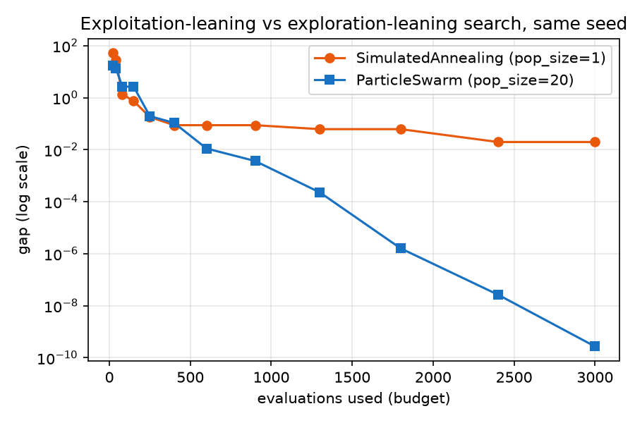
The sigma comparison above holds one algorithm fixed and varies a
parameter. The figure below contrasts two DIFFERENT algorithms that sit at
opposite ends of this same spectrum by design: SimulatedAnnealing
(pop_size=1, a single trajectory that commits hard to descending once
cooled — exploitation-leaning) and ParticleSwarm (pop_size=20, a
population sharing one global-best attractor — exploration-leaning until
its particles converge together):
The trade-off as a diagram
flowchart LR
    subgraph small["sigma = 0.05 (exploitative)"]
      S1(("current\npoint")) -.->|"small Gaussian\nstep"| S2(("tight cluster\nof offspring"))
    end
    subgraph large["sigma = 2.0 (explorative)"]
      L1(("current\npoint")) -.->|"large Gaussian\nstep"| L2(("wide-spread\noffspring"))
    end
    small --> CONV["fast, but risks\na local optimum"]
large --> COVER["slower to refine, but\ncovers more of the space"]Next
- Encodings and search spaces covers the other modeling decision every problem author makes: what a candidate point actually is.