Reading convergence curves

A convergence curve plots an algorithm's best-so-far fitness against evaluations used. It is the standard way to look at how a run actually behaved, not just where it ended up — two runs with the same final best_f can have gotten there completely differently (one steady, one stuck-then- jumping), and that difference matters when choosing an algorithm or a budget.

The curve, rendered

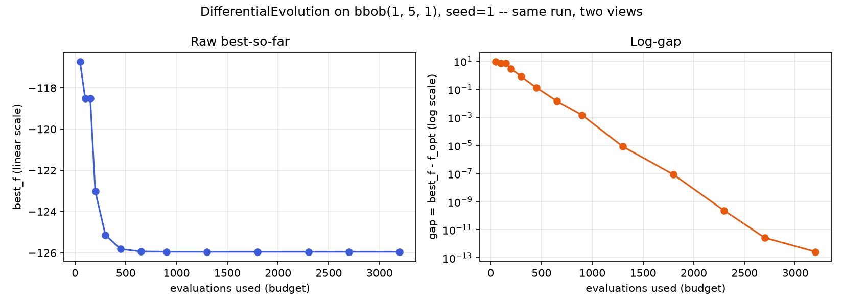
docs/scripts/fig_budget_anytime_curve.py runs exactly the scenario walked through by hand below (DifferentialEvolution(pop_size=20) on bbob(1, 5, 1), seed=1) at a denser set of budgets, plotted both ways — raw best-so-far and log-gap, side by side:

Anytime behavior, read without a plot

Because sezgi runs are deterministic under a fixed (problem, budget, seed) (see Determinism and the RNG model), four independent same-seeded runs at increasing budgets line up with one run's own trajectory here — but only because every budget below is a whole multiple of the population size (each run completes whole generations) and DifferentialEvolution's generator does not adapt to the budget. At a budget that cuts a generation short, or with a budget-adaptive algorithm such as LSHADE, independent runs can diverge from the long run's prefix (the quickstart's convergence section shows a concrete counterexample):

import sezgi

problem = sezgi.bbob(1, 5, 1)
seed = 1

# Four independent same-seeded runs. They reproduce one long run's
# trajectory here because each budget completes whole generations
# (multiples of pop_size=20) and this generator is not budget-adaptive.
for budget in (100, 300, 900, 2700):
    result = sezgi.DifferentialEvolution(pop_size=20).run(problem, budget=budget, seed=seed)
    print(f"budget={budget:5d} best_f={result.best_f:12.6g} gap={result.gap:12.6g}")

budget= 100 best_f= -118.504 gap= 7.44563 budget= 300 best_f= -125.137 gap= 0.813184 budget= 900 best_f= -125.948 gap= 0.00145279 budget= 2700 best_f= -125.95 gap= 2.70006e-12

Reading this table: in absolute terms the gap's improvement shrinks each step (7.45 → 0.81 → 0.0015 → ~0) — the curve flattens toward a floor, not a stall. But on a log scale (the natural scale for a gap approaching zero) the rate is not slowing down at all: roughly one order of magnitude between budget=100 and 300, then over two orders of magnitude between 300 and 900, then over eight between 900 and 2700 — the relative rate of improvement is accelerating here, which is exactly the fast local convergence a differential-evolution-style search shows once it is inside the right basin. A plateau approaching a floor still describes the absolute-scale shape, but "diminishing returns" would be the wrong read of the log-scale one. Whether the floor itself means "converged" or "stuck" cannot be told from either view alone; it depends on whether the floor is close to the problem's known optimum (as it is here, f_opt for BBOB f1 is known) or far from it.

Three honest ways to view the same run

• Raw best-so-far vs. evaluations — the direct view above; useful for seeing absolute progress, but a log-scale y-axis is usually needed once the gap gets small, since linear scale flattens everything past the first big drop.
• Log-gap vs. evaluations (best_f - f_opt, log-scaled) — makes the "orders of magnitude per generation" behavior in the table above directly visible as roughly straight-line segments.
• ECDF (empirical cumulative distribution of hitting-times) — sezgi.ecdf(log_root, targets=...) reads back an on-disk IOH-format log tree (written via run(..., log_dir=...) or run_experiment(..., log_dir=...)) and reports, across many runs and precision targets, the proportion that have reached each target by a given evaluation count — the standard way to summarize anytime performance over many seeds at once, rather than reading one curve at a time. See sezgi.read_ioh_records/sezgi.coco_export for the rest of that logging surface.

The shape of a plateau, sketched

flowchart LR
    A["evals=100\nbest_f far from optimum"] -->|"big early drop"| B["evals=300\nbest_f much closer"]
    B -->|"smaller drop"| C["evals=900\nbest_f very close"]
    C -->|"tiny drop"| D["evals=2700\nbest_f at the floor"]

    D --> Q{"Is the floor near\nthe known optimum?"}
    Q -->|yes| CONV["Converged --\nmore budget won't help much"]
    Q -->|no| STUCK["Stuck at a local optimum --\nmore budget alone won't fix this"]

Next

• Engine flow opens the architecture section: exactly what the Rust engine does, once per generation, to produce the numbers this whole Learn track has been printing.