ANFIS

An adaptive-network-based fuzzy inference system (ANFIS, Jang 1993) is a first-order Sugeno system whose membership functions and rule consequents are learned from numeric data. Use it to fit a smooth input-output map from samples while keeping the result readable as fuzzy rules: after training, to_sugeno hands you an ordinary SugenoFIS.

Architecture

bulanik implements the grid-partition form.

• Each input \(i\) has its own set of membership functions, Gaussian or generalized bell (mf="gaussian" or "bell"), with \(n_i\) terms.
• The rules are all combinations of one term per input, in itertools.product order, so \(n_1 n_2 \cdots\) rules. AND is the product.
• Rule \(r\) has a linear consequent \(p_r \cdot x + r_r\).

For an input vector \(x\), with \(w_r(x) = \prod_i \mu_{i,k_i(r)}(x_i)\) the firing strength of rule \(r\), the output is

\[ f(x) = \sum_r \bar w_r(x)\,(p_r \cdot x + r_r), \qquad \bar w_r = \frac{w_r}{\sum_s w_s}, \]

with \(\mu(x) = \exp\bigl(-(x - c)^2 / (2\sigma^2)\bigr)\) for gaussian and \(\mu(x) = 1 / (1 + |(x - c)/a|^{2b})\) for bell. The normalisation \(\bar w_r\) is computed in the log domain (a max-shifted softmax), so a sample far from every centre never gives \(0/0\); the result equals the plain ratio up to rounding.

In Jang's five-layer network these are: (1) fuzzify each input with its terms, (2) multiply the memberships of a rule (its firing strength \(w_r\)), (3) normalise to \(\bar w_r\), (4) apply the linear consequent \(\bar w_r (p_r \cdot x + r_r)\), (5) sum over the rules.

Initial centres are evenly spaced over each input's range, Gaussian \(\sigma\) and bell \(a\) are \((hi - lo) / (2(n - 1))\), bell \(b\) is 2, and all consequents are 0. Training is deterministic: there is no random initialisation, so the same data and options always give the same model.

Because the rule count is a product, the grid grows fast. More than 27 rules emits a UserWarning; more than 1024 raises ValueError unless you pass allow_large=True. For many inputs, use few terms each (2 or 3).

Training: hybrid least squares plus gradient descent

fit(X, y, epochs=50, method="hybrid", lr=0.01, ridge=1e-8) returns the training RMSE after each epoch (also stored as history) and continues from the current parameters.

method="hybrid" (Jang's rule, the default) alternates two things:

1. With the premise parameters (centres, widths) fixed, the output is linear in the consequent parameters, so all of them are solved at once by ridge least squares (normal equations, in pure Python). This runs before the first epoch and after every premise step, so a fitted model always ends on solved consequents.
2. One batch gradient step per epoch moves the premise parameters.

method="gradient" takes one batch gradient step on all parameters per epoch.

Hybrid learning usually converges in a few epochs because the hard part, the consequents, is solved exactly. The least-squares step works on inputs normalised to \([0, 1]\) over each input's range and maps the solution back, so it does not depend on the offset or scale of the data. The gradient step lr is not scale-invariant: rescaling an input changes the effective step.

lr is the largest step tried, not the step taken. A step that would raise the training RMSE is halved until it does not, and the next epoch starts from twice the step taken, up to lr. So history does not rise, apart from the small effect of ridge in hybrid training, and a too-large lr costs extra evaluations rather than the fit. A step that finds no descent after 60 halvings is dropped, which means lr is far too large, and fit warns.

import math
from bulanik.anfis import ANFIS

def sinc(t):
    return 1.0 if t == 0 else math.sin(t) / t

xs = [-10 + 20 * i / 40 for i in range(41)]
X, y = [[x] for x in xs], [sinc(x) for x in xs]

model = ANFIS(1, 5, ranges=[(-10, 10)])          # one input, five terms: five rules
print(model.n_rules, "rules; RMSE before training:", round(model.rmse(X, y), 3))
history = model.fit(X, y, epochs=20)
print("after epoch 1:", round(history[0], 5), " after 20:", round(history[-1], 5))

gradient = ANFIS(1, 5, ranges=[(-10, 10)])
losses = gradient.fit(X, y, epochs=20, method="gradient", lr=0.05)
print("gradient only, 20 epochs:", round(losses[-1], 3))
print(round(model.predict([[0.0]])[0], 4), "vs sinc(0) = 1")

5 rules; RMSE before training: 0.385
after epoch 1: 0.00379  after 20: 0.00379
gradient only, 20 epochs: 0.316
0.9951 vs sinc(0) = 1

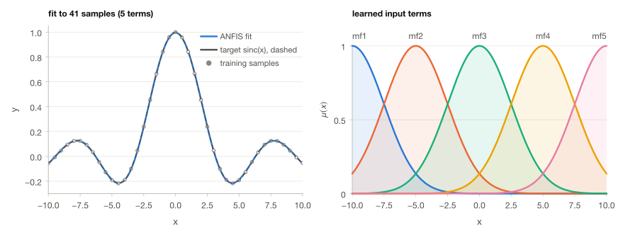
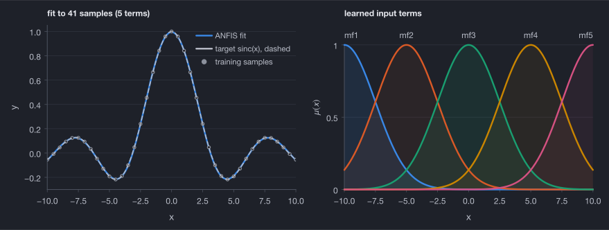
A one-input ANFIS with five Gaussian terms fitted to 41 samples of \(\operatorname{sinc}(x)\) by the hybrid method. The fitted curve is drawn by plot.surface and the terms by plot.variable, both from the exported Sugeno system.

On a smooth target the hybrid fit is essentially done after the first epoch (the history above is nearly flat); later epochs change almost nothing. The fit is only as good as the grid: with three terms the same data leave a visible error, and the number of terms is the main model-selection knob.

Numerical safeguards

• Ridge fallback. The least-squares solve adds ridge to the diagonal of the normal matrix. If it is still singular to working precision (for example ridge=0 with a rank-deficient design, such as every sample at one input value), the ridge is raised automatically, ten times per retry from at least \(10^{-12}\) times the largest diagonal entry, instead of failing.
• Floors. After each step widths (\(\sigma\), bell \(a\)) are floored at MIN_WIDTH * span of their input (MIN_WIDTH) and bell \(b\) at MIN_B.
• Step halving. A step that would make any parameter or the training RMSE non-finite is halved until it does not, and skipped after 60 halvings (a non-finite gradient is skipped at once). A skipped epoch repeats the previous RMSE in the history, and a fit that skipped any step emits one RuntimeWarning with the count.

import warnings
from bulanik.anfis import ANFIS

X = [[i / 10] for i in range(21)]
y = [x[0] ** 2 for x in X]

model = ANFIS(1, 3, ranges=[(0, 2)])
with warnings.catch_warnings(record=True) as caught:
    warnings.simplefilter("always")
    history = model.fit(X, y, epochs=4, method="gradient", lr=1e300)   # absurd step size
print(history)                                  # every step skipped: the RMSE never moves
print(caught[0].category.__name__, "-", caught[0].message)

same = ANFIS(1, 3, ranges=[(0, 2)])
print(same.fit([[1.0]] * 5, [1.0] * 5, epochs=2, ridge=0))   # singular normal matrix: ridge raised

[1.8550651381195935, 1.8550651381195935, 1.8550651381195935, 1.8550651381195935]
RuntimeWarning - ANFIS.fit skipped 4 of 4 gradient steps: none lowered the error within 60 halvings or the gradient was not finite; lower lr
[7.717160244169463e-13, 7.717160244169463e-13]

Prediction and extrapolation

predict(X) takes rows of n_inputs numbers. The model is only trained inside its ranges (given at construction or taken from the data at the first fit). An input outside them still gets a prediction, but because the consequents are linear it extrapolates and can be far off, and one ExtrapolationWarning (a RuntimeWarning) names the first offending sample. rmse(X, y) scores a data set.

import warnings
from bulanik.anfis import ANFIS, ExtrapolationWarning

X = [[i / 10] for i in range(21)]
y = [x[0] ** 2 for x in X]
model = ANFIS(1, 3, ranges=[(0, 2)])
model.fit(X, y, epochs=5)
print(model.predict([[1.0], [1.5]]))
with warnings.catch_warnings(record=True) as caught:
    warnings.simplefilter("always")
    print(model.predict([[4.0]]))               # the target would be 16
print(caught[0].category is ExtrapolationWarning, "-", caught[0].message)

[1.0123147137644106, 2.2395266350875462]
[10.902983735691624]
True - ANFIS.predict: sample 0 has input 0 = 4 outside the trained range [0, 2]; the prediction extrapolates

Exporting to a Sugeno system

to_sugeno(input_names=None, output_name="y") returns a SugenoFIS with and_method="prod": one variable per input over its range with terms mf1..mfn, and one Linear output term r1..rR per rule. It reproduces predict inside the ranges, so you can read the learned rules, evaluate them, plot them, or tune them further.

from bulanik.anfis import ANFIS

X = [[i / 10] for i in range(21)]
y = [x[0] ** 2 for x in X]
model = ANFIS(1, 3, ranges=[(0, 2)])
model.fit(X, y, epochs=5)

fis = model.to_sugeno(["x"])
for rule in fis.rules:
    print(rule)
print(fis.outputs[0].functions["r2"])           # the learned first-order consequent
print(fis.evaluate({"x": 1.0})["y"], model.predict([[1.0]])[0])

IF x IS mf1 THEN y IS r1
IF x IS mf2 THEN y IS r2
IF x IS mf3 THEN y IS r3
Linear({'x': 1.9999648691301257}, -0.9051244307788873)
1.0123147137644104 1.0123147137644106

The two differ in exactly two ways. The exported system rejects inputs outside the ranges (a ValueError) where predict extrapolates with a warning. And where every membership underflows to 0 in plain floating point, predict still answers (it normalises in the log domain) while the exported system raises NoRuleFiredError.

Training with sezgi

fit is gradient-based. For a derivative-free search, the optional sezgi bridge exposes an ANFIS as a sezgi problem (train_anfis) and trains it with a sezgi optimiser: see the sezgi bridge page and the example 16 ANFIS with sezgi.

Pitfalls

Too many rules. The grid is the product of the term counts: 3 inputs with 4 terms is 64 rules (a UserWarning above 27), and 11 inputs with 3 terms is 177 147, refused with a ValueError. Reduce the terms or the inputs before reaching for allow_large=True.

Constant inputs. If ranges is not given, each input's range comes from the data, so an input that is constant in X has no range and fit raises ValueError. Pass ranges explicitly.

Few samples, many parameters. A 1-input model with \(n\) terms has \(2n\) premise parameters (Gaussian; \(3n\) for bell) and \(2n\) consequent parameters; fitting it to fewer samples than that overfits or leaves the least squares under-determined (the ridge fallback hides the singularity but not the over-fitting).

Do not read extrapolated predictions. The ExtrapolationWarning is not noise: linear consequents far outside the data can be wildly wrong. Clip inputs yourself, or train on a range that covers deployment.

lr depends on the data scale. The same lr can be gentle for inputs in \([0, 1]\) and far too large for inputs in \([0, 1000]\). The descent check stops that from harming the fit, but a history that stays flat can still mean a poor start for the premise. If a RuntimeWarning reports skipped steps, lower lr.

from bulanik.anfis import ANFIS

def show(make):
    try:
        print(make())
    except Exception as error:
        print(f"{type(error).__name__}: {error}")

show(lambda: ANFIS(0, 2))
show(lambda: ANFIS(2, [2, 3, 4]))
show(lambda: ANFIS(1, 2, mf="triangular"))
show(lambda: ANFIS(11, 3))
show(lambda: ANFIS(1, 2).fit([[1.0], [1.0]], [0.0, 1.0]))
show(lambda: ANFIS(1, 2, ranges=[(0, 1)]).fit([[0.5]], [1.0], epochs=0))
show(lambda: ANFIS(1, 2, ranges=[(0, 1)]).fit([[0.5], [0.6]], [1.0]))
show(lambda: ANFIS(1, 2, ranges=[(0, 1)]).fit([[0.5]], [1.0], method="newton"))
show(lambda: ANFIS(1, 2).to_sugeno())
show(lambda: ANFIS(1, 2, ranges=[(0, 1)]).to_sugeno(["a", "b"]))

ValueError: n_inputs must be an integer >= 1, got 0
ValueError: n_mfs must be an integer >= 1 or 2 such integers, got [2, 3, 4]
ValueError: unknown mf 'triangular' for ANFIS; valid: gaussian, bell
ValueError: grid partition gives 177147 rules (> 1024); pass allow_large=True to build it anyway
ValueError: input 0 is constant in X (1); pass ranges=... explicitly
ValueError: epochs must be an integer >= 1, got 0
ValueError: got 2 samples but 1 targets
ValueError: unknown method 'newton' for ANFIS.fit; valid: hybrid, gradient
RuntimeError: ANFIS has no input ranges yet: pass ranges=... or call fit first
ValueError: input_names needs 1 names, got 2

See also

• Sugeno and Tsukamoto for the model to_sugeno returns, and sezgi bridge for derivative-free training.
• API: bulanik.anfis, bulanik.plot.
• Examples: 15 ANFIS sinc (a two-input grid and the Sugeno export), 16 ANFIS with sezgi.
• Jang (1993), "ANFIS: adaptive-network-based fuzzy inference system", IEEE Transactions on Systems, Man, and Cybernetics.